Rtglm: package overview

Rtglm provides a way to

1. Reproduce results of EpiEstim
2. Rely on GAM for temporal smoothing of Rt
3. Rely on GAM for spatial smoothing of Rt

Installing the package

To install the current stable, CRAN version of the package, type:

To benefit from the latest features and bug fixes, install the development, github version of the package using:

devtools::install_github("pnouvellet/Rtglm",build = TRUE)
devtools::install_github("pnouvellet/MCMCEpiEstim",build = TRUE)

Note that this requires the package devtools installed. We then install few additional useful package for this vignette.

rm(list=ls())
library(Hmisc)
library(EpiEstim)
library(incidence)
library(projections)
library(ggplot2)
library(Rtglm)
library(MCMCEpiEstim)
library(sf)

Reproducing EpiEstim results in a Rt.glm framework

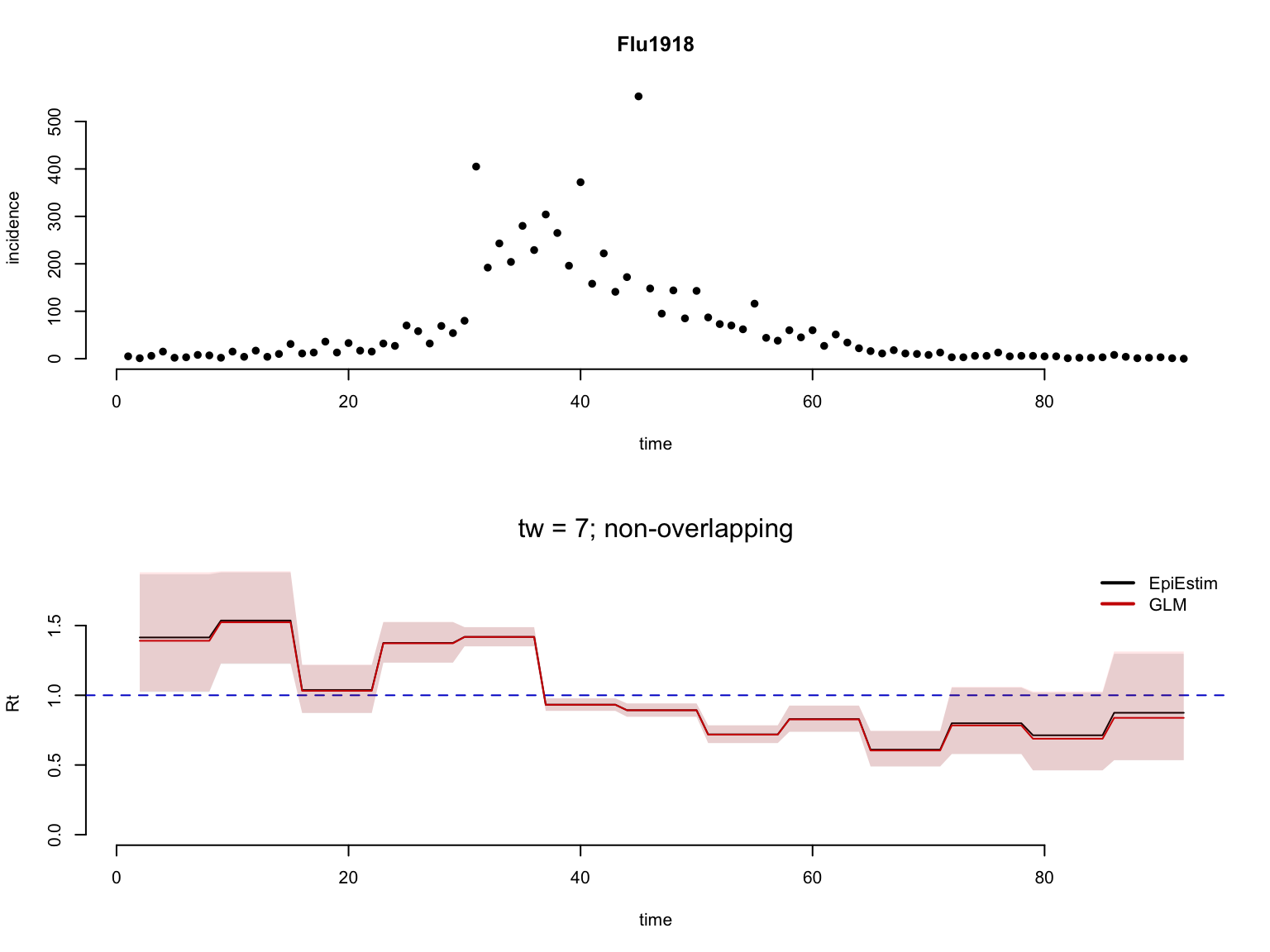
First, we load data (from EpiEstim), e.g. the daily incidence of the 1918 influenza in Baltimore.

# load data
data <- data(Flu1918)

# make a column for local and imported cases in incidence
Flu1918$incidence <- data.frame(local = Flu1918$incidence,
                                imported = 0)
# assume first case is imported and others are local cases.
Flu1918$incidence$imported[1] <- Flu1918$incidence$local[1]
Flu1918$incidence$local[1] <- 0
    
# plot incidence
plot(rowSums(Flu1918$incidence),
     main = 'Flu 1918', bty = 'n', pch = 16,
     ylab = 'incidence', xlab = 'time')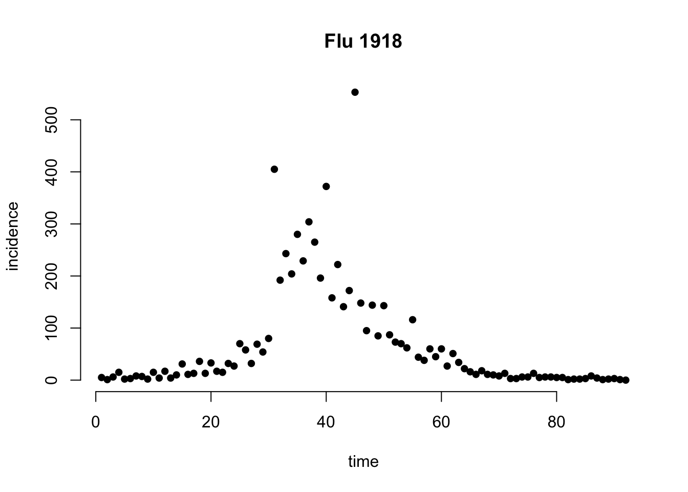

EpiEstim estimate

First, we set the prior distribution for Rt

# prior distribution for Rt, gamma distribution.
mean_prior = 5
std_prior = 5
para_prior <- epitrix::gamma_mucv2shapescale(mu = mean_prior,cv = std_prior/mean_prior)
hist(rgamma(n = 1e3,shape = para_prior$shape, scale = para_prior$scale),
     main = 'prior dist. Rt', bty = 'n', 
     ylab = 'dist', xlab = 'Rt' )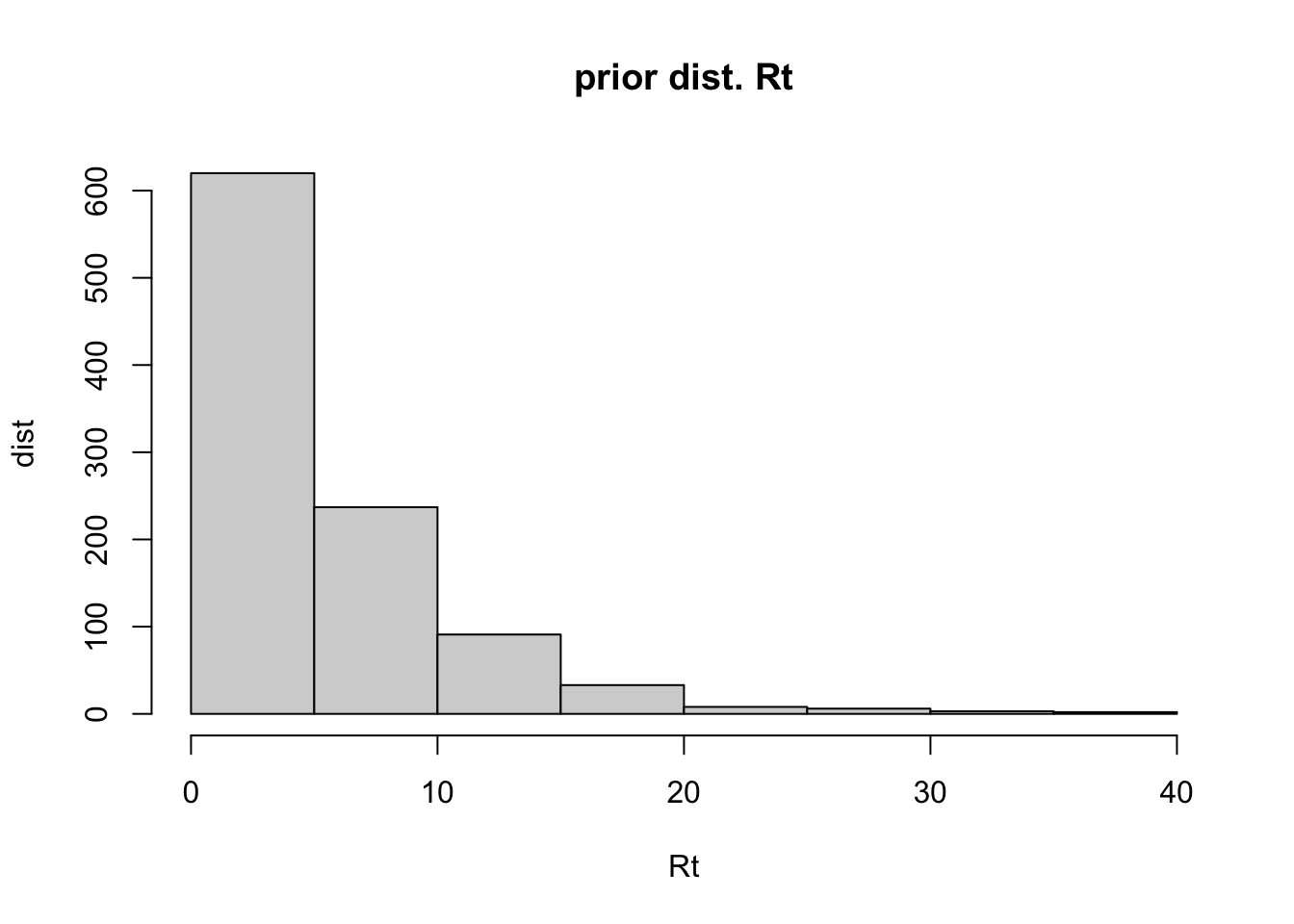

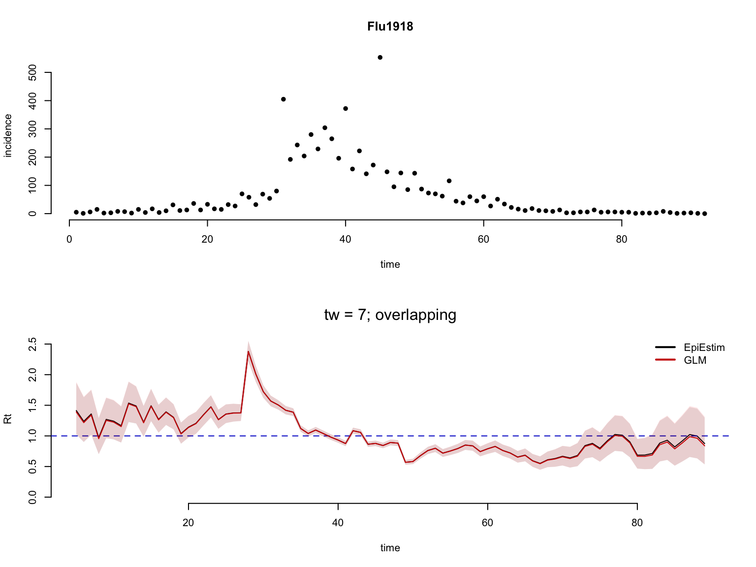
Here we run EpiEstim using an Rtglm wrapper to obtain standardized output. the wrapper is part of Rtglm. We run EpiEstim with a 7 day time-window, with and without overlapping time-windows.

# time windows
t_window <- c(7,7) # 7 days time-windows
overlap <- c(TRUE,FALSE) # overlapping or non-overlapping time-windows

# output
Rt_EpiEstim <- list()

for(i in 1:length(t_window)){ # estimate Rt for all time-windows above
  
  res <- Rtglm::EpiEstim_wrap(I_incid = Flu1918$incidence, 
                              si_distr = Flu1918$si_distr, 
                              t_window = t_window[i], 
                              overlap = overlap[i],
                              mean_prior = mean_prior, std_prior = std_prior)
  
  Rt_EpiEstim[[i]] <- res
}

Rt.glm estimate

# output
Rt_glm <- list()

# same analyses but using the GLM formulation
for(i in 1:length(t_window)){
  res <- Rtglm::glm_Rt_wrap(I_incid = Flu1918$incidence, 
                            si_distr = Flu1918$si_distr, 
                            t_window = t_window[i], 
                            overlap = overlap[i])
  
  
  Rt_glm[[i]] <- res
}

Compare estimates

Plot the resulting Rt estimates.

layout(matrix(c(1,1,1,1,2,2,2,2),nrow = 4, ncol = 2, byrow = TRUE))

for(i in 1:length(t_window)){
  # plot incidence
  plot(rowSums(Flu1918$incidence),
       main = 'Flu1918', bty = 'n', pch = 16,
       ylab = 'incidence', xlab = 'time')
  
  # plot EpiEstim and Rt.glm estimates
  a <- Rt_EpiEstim[[i]]$Rt[,c('t','Mean','low_Quantile','high_Quantile')]
  b <- Rt_glm[[i]]$Rt[,c('t','Mean','low_Quantile','high_Quantile')]
  
  res <- plot_compare2Rt(a = a, b = b,
                         t_window = t_window[i],
                         overlap = overlap[i],
                         Corr=TRUE)
}

Estimating Rt with a temporal smoothing

First, we characterising the serial interval.

si <- Flu1918$si_distr
I0 <- incidence::as.incidence(x = 30, dates = 1, interval = 1)

Then, we simulate an Rt trend over time, here we choose a sinusoidal pattern with a period of 30days and amplitude of 0.2 centered on 1.

x <- 1:101
B <- 30
A <- .2
Rt <- data.frame(t = x, 
                  Rt = A*sin((x+4)*2*pi/B)+1)

plot(Rt$t,Rt$Rt,type='l',lwd = 3,
     bty = 'n', xlab = 'Rt', ylab = 'time', ylim = c(0,1.5),
      xaxt='n',  yaxt='n', cex.lab=1.5)
axis(side = 1, at = c(0,50,100))
axis(side = 2, at = c(0,.50,1, 1.5))
abline(h = 1,col = 'red3', lty = 2)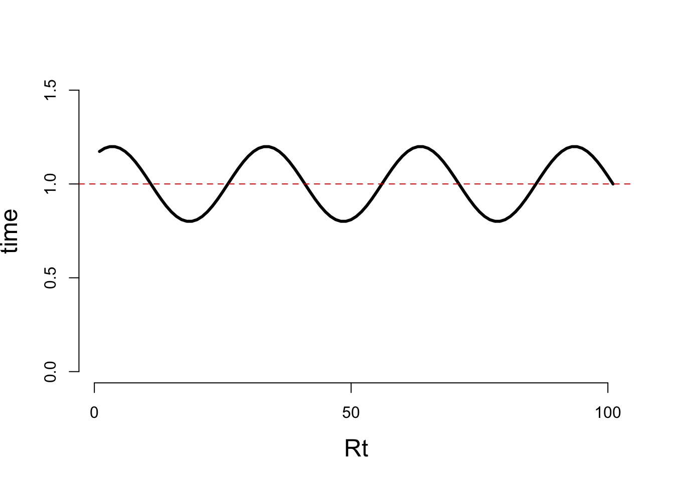

Simulate incidence

In simulating incidence, we make use of code available in MCMCEpiEstim R-package.

set.seed(1)
# make simulated incidence for a given initial conditions (I0), an Rt pattern (Rt), 
# for a single location (n_loc = 1), using a Poisson offspring distribution (model), 
# and assuming all cases are reported (below: p = 1).
res <- MCMCEpiEstim::project_fct(I0 = I0,
                                 Rt = Rt,
                                 n_loc = 1,
                                 t_max = nrow(Rt),
                                 si = si,
                                 p = 1,
                                 model = 'poisson')

sim_incidence <- res$I_true
# visualise the simulated incidence
plot(sim_incidence[,2],
     main = 'simulated incidence', bty = 'n', pch = 16,
     ylab = 'incidence', xlab = 'time')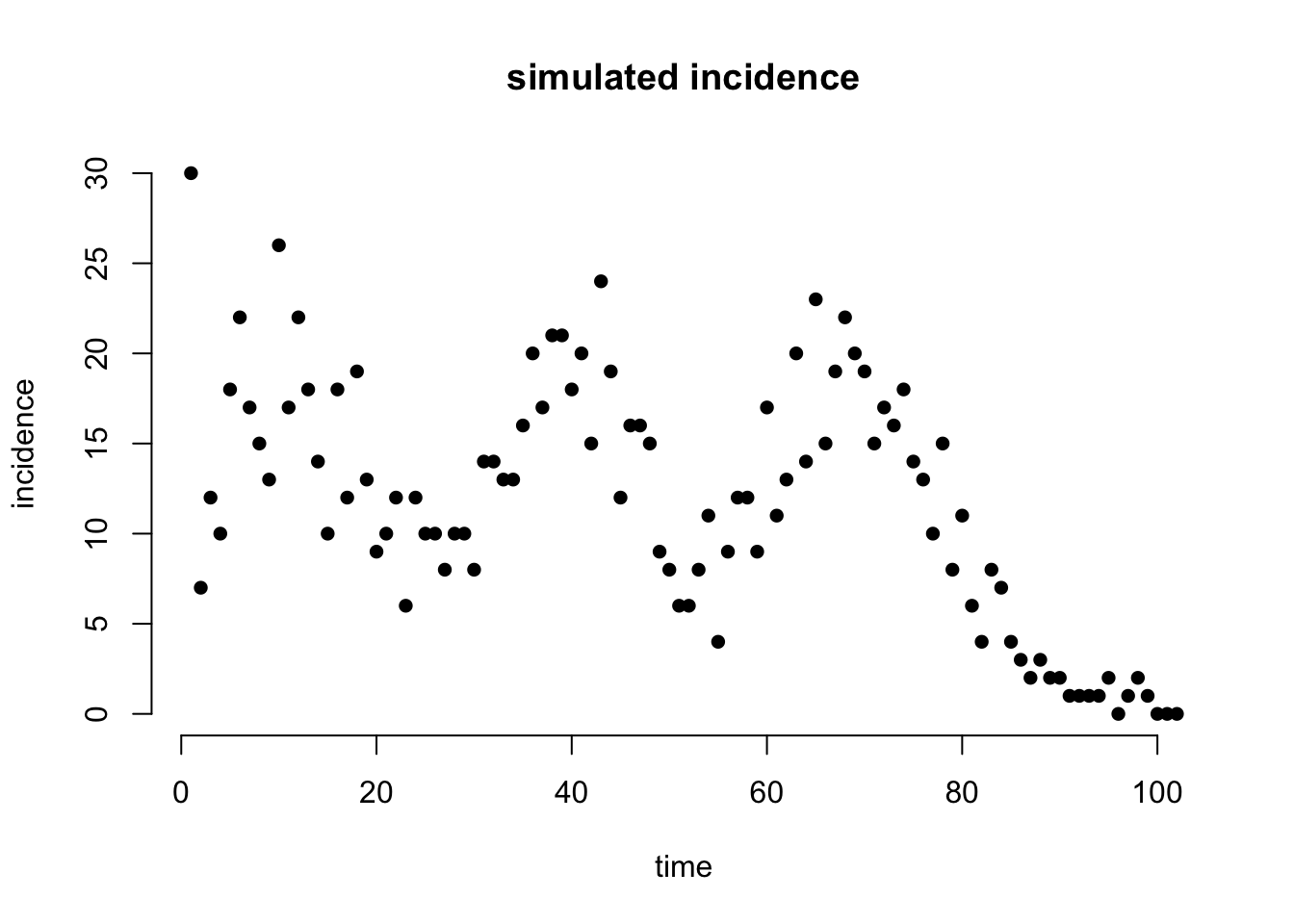

# format incidence with local and imported cases as before.
data <- data.frame(local = c(0,sim_incidence[2:nrow(sim_incidence),2]),
                   imported = c(sim_incidence[1,2],rep(0,nrow(sim_incidence)-1) ))

Estimate Rt using EpiEstim

mean_prior = 5
std_prior = 5

# time windows
t_window <- 7 
overlap <- TRUE

# output
Rt_EpiEstim <- Rtglm::EpiEstim_wrap(I_incid = data,
                                    si_distr = si,
                                    t_window = t_window,
                                    overlap = overlap,
                                    mean_prior = mean_prior, std_prior = std_prior)

Estimate Rt using Rtglm

# output
Rt_gam <- Rtglm::gam_Rt_wrap(I_incid = data,
                             si_distr = si)

Compare estimates

Visualise the estimated Rt trends estimated with EpiEstim, and with Rtglm using a temporal smooth.

layout(matrix(c(1,1,1,1,2,2,2,2),nrow = 4, ncol = 2, byrow = TRUE))

# plot incidence
plot(rowSums(data),
     main = 'simulated incidence', bty = 'n', pch = 16,
     ylab = 'incidence', xlab = 'time')

# plot simulated Rt
ylim <- c(0,1.5)
plot(Rt$t, Rt$Rt,type = 'l', lwd=2, 
     ylim = ylim,bty = 'n',
     xlab = 'time',ylab = 'Rt',
     main = '')

# plot EpiEstim estimates
f <- which( !is.na(Rt_EpiEstim$Rt$Mean) ) # remove time-points where Rt cannot be estimated
lines(Rt_EpiEstim$Rt$t[f], Rt_EpiEstim$Rt$Mean[f],col='red3')
polygon(c(Rt_EpiEstim$Rt$t[f],rev(Rt_EpiEstim$Rt$t[f])),
        c(Rt_EpiEstim$Rt$low_Quantile[f],
          rev(Rt_EpiEstim$Rt$high_Quantile[f])), 
        col = rgb(1,0,0,.1), border = NA)

# plot Rt.glm estimates
f <- which( !is.na(Rt_gam$Rt$Mean) ) # remove time-points where Rt cannot be estimated
lines(Rt_gam$Rt$t[f], Rt_gam$Rt$Mean[f],col='green4')
polygon(c(Rt_gam$Rt$t[f],rev(Rt_gam$Rt$t[f])),
        c(Rt_gam$Rt$low_Quantile[f],
          rev(Rt_gam$Rt$high_Quantile[f])), 
        col = rgb(0,1,0,.2), border = NA)

legend('bottomleft',legend = c('simulated','EpiEsitm','Rt.gam'), 
       lwd=1, col = c('black','red3','green4'), bty = 'n')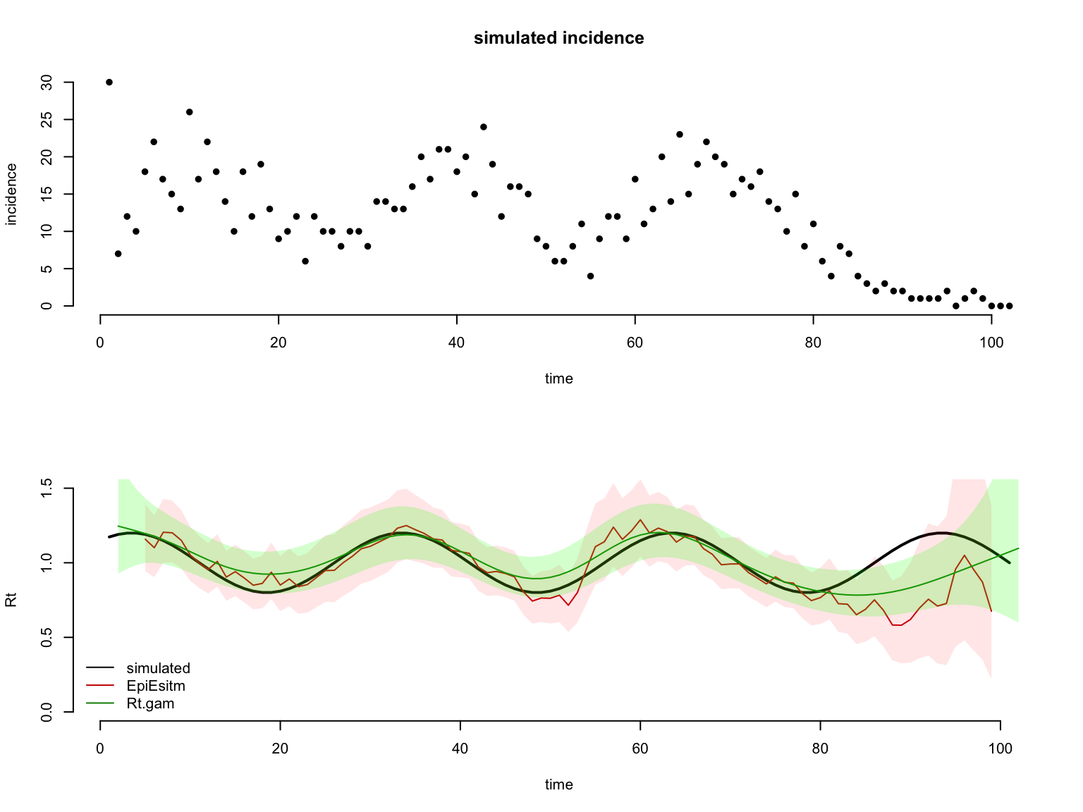

Spatial smoothing

We first load a map of the Unitary Authorities of the United Kingdom.

if (file.exists('ukMap.rds')){
  uk <- readRDS('ukMap.rds')
}else{
  # Define the raw URL
  rds_url <- "https://raw.githubusercontent.com/pnouvellet/Rtglm/master/vignettes/ukMap.rds"
  # Temporary file path
  temp_file <- tempfile(fileext = ".rds")
  # Download the file
  download.file(rds_url, temp_file, mode = "wb")
  # Read the RDS file
  uk <- readRDS(temp_file)
}
class(uk)

## [1] "sf"         "data.frame"

Simulate Rt trends over space

We use the same method as in: Rtglm: Unifying estimation of the time-varying reproduction number, Rt , under the Generalised Linear and Additive Models.

In Summary, We construct a kernel formed of 3 distinct 2-dimension Normal distributions, with means chosen randomly among centroid of the UA of the UK and with variance randomly chosen between 0.5 and 2.

library(mvtnorm)
set.seed(1)

# range of simulated Rt
Rt_min_max <- data.frame(max = 2,
                        min = 0.5)

# range of the variance of the bi-variate Normals
var_range <- c(.5,2)

# locations of 3 peak in Rt and associated variances
r_loc <- sample(x = 1:nrow(uk),size = 3,replace = TRUE)
Mus <- list(c(uk$cent.x[r_loc[1]],uk$cent.y[r_loc[1]]),
            c(uk$cent.x[r_loc[2]],uk$cent.y[r_loc[2]]),
            c(uk$cent.x[r_loc[3]],uk$cent.y[r_loc[3]]))
Sigmas <- runif(n = 3, min = var_range[1], max = var_range[2])

# simulate Rt
R_true <- data.frame(GID_2 = uk$GID_2,
                     cent.x = uk$cent.x, cent.y = uk$cent.y,
                     Rt = NA)

# simulate Rt
R_true$Rt <- Rtglm::kernel_rt(map = uk,
                       mu = Mus, sigma = Sigmas,
                       Rt_min_max = Rt_min_max)

Optional plot to visualise the true Rt

temp <- merge(uk,R_true)

ggplot(temp, aes(fill = Rt)) +
  ggplot2::geom_sf() +
  scale_fill_viridis_c()

Simulate incidence

We first define some useful function to back-calculate incidence expected given Rt and a total incidence.

# function that recovers growth rate (r) from Reproduction number (R) and serial interval
# taken from Walling and Lipsitch 2006
r_2_R <- function(r){
  R <- 1/sum(exp(-r*0:(length(si)-1))*si)
  return(R)
}

# r_2_R(r = -0.5)
# function to numerically find the root of equation above, e.g. find r given R and the serial interval
findRoot <- function(r,R){
  R_check <- r_2_R(r)
  return( (R_check - R)^2 )
}
# test
# r <- optim(par = 0, fn = findRoot, method = 'BFGS', hessian=TRUE, R = 2 )$par

simulate incidence

ini_I <- I_sim <- list()
I0 <- 30
t_sim <- 5 # simulate 5 days of incidence to be used in the inference

# initialise incidence according to Rt, prior to the period of inference.
for (i in 1:nrow(uk)){   # do it for each locations
  R <- R_true$Rt[i] # location specific Rt
  # find growth rate associated with Rt above
  ini_r <- optim(par = 0, fn = findRoot,
                 method = 'BFGS',
                 hessian=TRUE, R = R )$par
  # we simulate 10 days incidence prior to inference period
  init_t <- 10
  # find the exponential growth/decline associated with Rt starting from 1 case
  temp <- exp(ini_r*1:init_t)
  # compute the associated overall infectivity
  temp2 <- EpiEstim::overall_infectivity(incid = temp,
                                         si_distr =  si)
  # adjust incidence such that if R=1, given the simulated incidence,
  # we would expect 30 cases on the first simulation day
  # on day 1 of simulation: E{I_11} = R* Sum{I{1:10}*si{10:1}}
  temp3 <- temp/temp2[init_t]*I0 
  # return integer incidence object
  ini_I[[i]] <-  incidence::as.incidence(x = round(temp3),
                                         dates = 1:init_t, interval = 1)
}

# now simulate some stochastic incidence given the above
for (i in 1:nrow(uk)){
  R <- R_true$Rt[i]
  # simulate incidence
  I <- as.data.frame(projections::project(x = ini_I[[i]],
                                          R = R,
                                          n_sim = 1, # number of simulation
                                          si = si[-1],
                                          n_days = t_sim,
                                          instantaneous_R = TRUE))
  
  
  d_incidence <- data.frame(t = c(1:ini_I[[i]]$timespan,I[,1]),
                            incidence = c(ini_I[[i]]$counts,I[,2]))
  
  # specify importation (e.g. the initialisation)
  I_corr <- data.frame(local = d_incidence$incidence,
                       imported = 0)
  # correct initial case as imported
  I_corr$imported[1:init_t] <- d_incidence$incidence[1:init_t]
  I_corr$local[1:init_t] <- 0
  
  
  I_sim[[i]] <- I_corr
}

Estimates using EpiEstim

By UA

We independently estimate one Rt for each UA.

res <-  data.frame(matrix(NA, nrow = nrow(uk), ncol = 5))
names(res) <-  c('Mean','Std',
                 'low_Quantile','Median','high_Quantile')

for (i in 1:nrow(uk)){
  
  res_EE <- Rtglm::EpiEstim_sp_wrap(I_incid = I_sim[[i]],
                                    si_distr = si,
                                    t_ini = init_t)
  
  
  res[i,] <- c(res_EE$R$Mean, res_EE$R$Std,
               res_EE$R$low_Quantile, res_EE$R$Median, res_EE$R$high_Quantile)
}

names(res) <- paste0('UA_',names(res))
R_UA <- res

By mid-grid

We compute the aggregated incidence within a grid comprising multiple UA. Then, as above, we independently estimate one Rt for each grid.

res <-  data.frame(matrix(NA, nrow = nrow(uk), ncol = 5))
names(res) <-  c('Mean','Std',
                 'low_Quantile','Median','high_Quantile')

unique_grid <- unique(uk$grid2)

for (i in 1:length(unique_grid)){
  # find which UA belong to the grid
  f <- which(uk$grid2 %in% unique_grid[i])
  # initialise incidence with the first UA belonging to the grid
  I_corr <- I_sim[[ f[1] ]]
  # add incidence from other UAs belong to the grid
  if(length(f)>1){
    for(l in 2:length(f)){
      I_corr <- I_corr+I_sim[[ f[l] ]]
    }
  }
  
  # estimate Rt for the grid
  resEE <- Rtglm::EpiEstim_sp_wrap(I_incid = I_corr,
                                   si_distr = si,
                                   t_ini = init_t)
  
  # save output
  res[f,] <- matrix(data = c(resEE$R$Mean, resEE$R$Std,
                             resEE$R$low_Quantile, resEE$R$Median,
                             resEE$R$high_Quantile), nrow = length(f), ncol = 5,
                    byrow = TRUE)
  
}

names(res) <- paste0('grid_',names(res))
R_grid <- res

Rt.glm estimate

Estimate Rt across space, using a smooth spatial function for Rt.

res_gam <- Rtglm::gam_Rt_sp_wrap(I_incid = I_sim,
                          si_distr = si,
                          x=uk$cent.x,
                          y=uk$cent.y)

res <- res_gam$Rt[,-1]
names(res) <- paste0('gam_',names(res))
R_gam <- res

Compare estimates

Visualise the results

maps of Rts

First, we prepare the dataframe for ggplot.

uk <- st_sf(cbind(uk,
              R_UA,
              R_grid,
              R_gam))

temp <- R_true[,c(1,4)]
names(temp)[2] <- 'R'

uk <- merge(uk,temp)

We plot the mean Rt estimates, using either EpiEstim at UA scale, at grid scale, and using Rtglm with a spatial smooth.

ggplot(uk, aes(fill = R)) +
  ggplot2::geom_sf() +
  ggtitle('Simulated Rt')+
  scale_fill_viridis_c(limits = c(0, 3),name = 'R',option = 'H') 

ggplot(uk, aes(fill = UA_Mean)) +
  ggplot2::geom_sf() +
  ggtitle('EpiEstim Rt - UA')+
  scale_fill_viridis_c(limits = c(0, 3),name = 'R',option = 'H') 

limits_x <- seq(min(uk$cent.x),max(uk$cent.x),length.out = 5)
limits_y <- seq(min(uk$cent.y),max(uk$cent.y),length.out = 5)

ggplot(uk, aes(fill = grid_Mean)) +
  ggplot2::geom_sf() +
  ggtitle('EpiEstim Rt - medium grid') +
  scale_fill_viridis_c(limits = c(0, 3),name = 'R',option = 'H') +
  geom_vline(xintercept=limits_x[-c(1,length(limits_x))], linetype="solid",col='red3')+
  geom_hline(yintercept=limits_y[-c(1,length(limits_x))], linetype="solid",col='red3')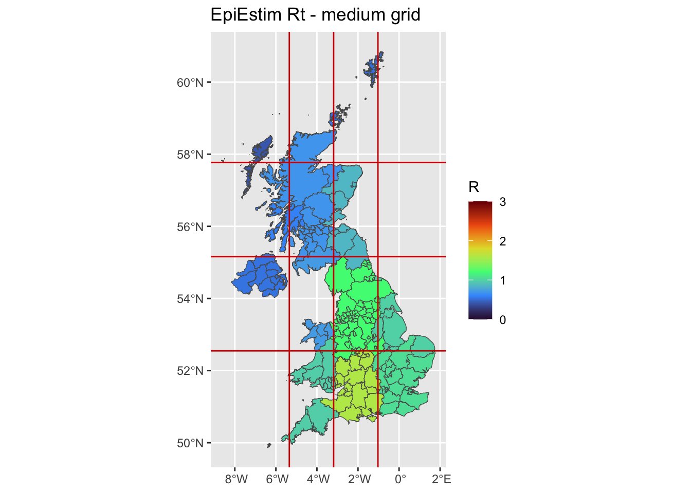 

ggplot(uk, aes(fill = gam_Mean)) +
  ggplot2::geom_sf() +
  ggtitle('GAM Rt') +
  scale_fill_viridis_c(limits = c(0, 3),name = 'R',option = 'H')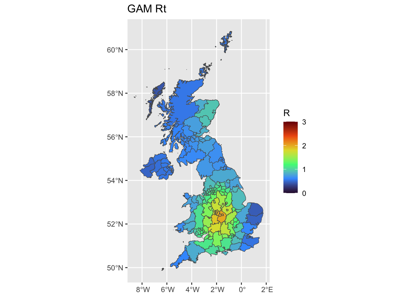  

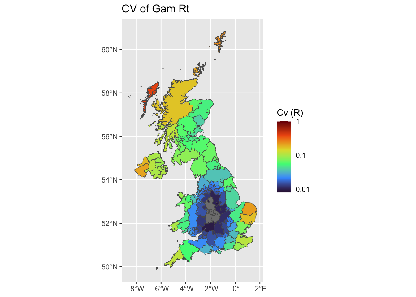
plot uncertainties maps (CV)

We plot the mean Coefficient of Variation estimates, using either EpiEstim at UA scale, at grid scale, and using Rtglm with a spatial smooth.

uk$UA_cvL <- log10(uk$UA_Std/uk$UA_Mean)
uk$grid_cvL <- log10(uk$grid_Std/uk$grid_Mean)
uk$gam_cvL <- log10(uk$gam_Std/uk$gam_Mean)

# range(c(temp$UA_cvL ,
#         temp$grid_cvL ,
#         temp$gam_cvL))

ggplot(uk, aes(fill = UA_cvL)) +
  ggplot2::geom_sf() +
  ggtitle('CV of EpiEstim Rt - UA')+
  scale_fill_viridis_c(limits = c(-2.1,0),name = 'Cv (R)',option = 'H',
                       breaks = c(-3,-2,-1,0), labels = 10^c(-3,-2,-1,0))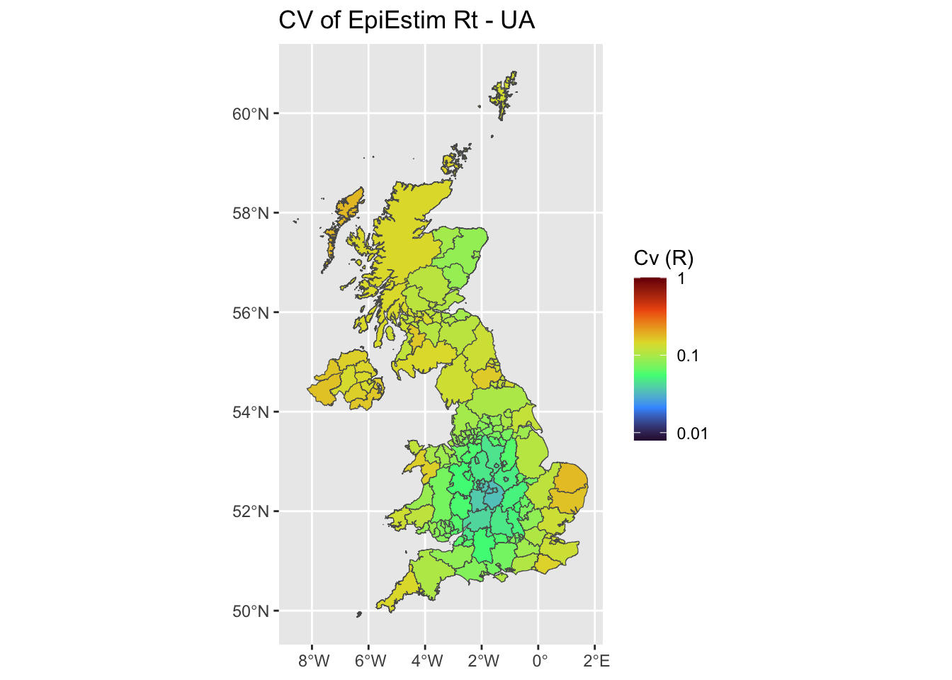 

ggplot(uk, aes(fill = grid_cvL)) +
  ggplot2::geom_sf() +
  ggtitle('CV of EpiEstim Rt - medium grid') +
  scale_fill_viridis_c(limits = c(-2.1,0),name = 'Cv (R)',option = 'H',
                       breaks = c(-3,-2,-1,0), labels = 10^c(-3,-2,-1,0)) +
  geom_vline(xintercept=limits_x[-c(1,length(limits_x))], linetype="solid",col='red3')+
  geom_hline(yintercept=limits_y[-c(1,length(limits_x))], linetype="solid",col='red3')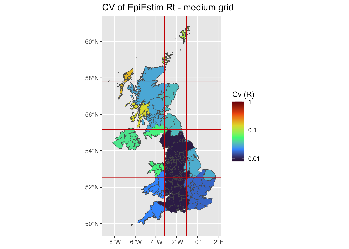 

ggplot(uk, aes(fill = gam_cvL)) +
  ggplot2::geom_sf() +
  ggtitle('CV of Gam Rt') +
  scale_fill_viridis_c(limits = c(-2.1,0),name = 'Cv (R)',option = 'H',
                       breaks = c(-3,-2,-1,0), labels = 10^c(-3,-2,-1,0))